People often use Excel to store lists of data which need to be ranked.
For example, you may use Excel to store information about your bowling team, and
you want to determine the ranks for players and scores. Excel provides a
worksheet function called
Simple Ranking
You can use the RANK function to return the rank of a value as it falls into a list of data. The rank of a value is simply the order in which it would appear if the list were sorted. The ranking can be done in either ascending or descending order. With descending order (the default), the highest value is given a rank of 1, the second highest is given a rank of 2, and so on. This is the most common method of ranking. It is what you would use to rank the scores of basketball players, where high scores indicate the better players. In an ascending ordered rank, the lowest score gets a rank of 1, the second lowest score gets a rank of 2, and so on. This is the type of ranking you would use to rank golf players, where the low scores indicate the better players.
One of the problems with the RANK function is that it assigns equal ranks to duplicate values. For example, suppose you have a list of ten numbers: 11, 22, 33, 44, 44, 44, 77, 88, 99, 111. The three entries with a value of 44 will all be given the same rank of 4, and the next largest entry, 77, will get the rank 7. There will be no values with the ranks of 5 or 6. This may cause a problem with your worksheet, depending on how you're using the rank values.
This section will describe the procedures for calculating Unique Ranks in both descending and ascending order. These formulas and sample data are illustrated in the following worksheet:
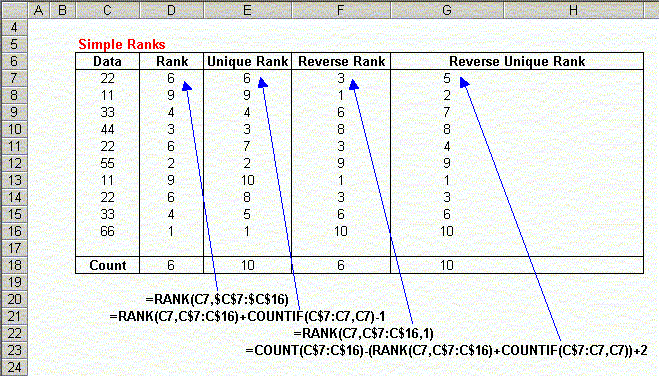
Unique Ranks
Using a simple worksheet formula, you can create unique ranks in a list. As you can see, there are duplicate ranks in column D of the sample worksheet. We have 3 ranks equal to 6, and none equal to 7 or 8. The following formula will compute unique ranks, as shown in column E of the sample worksheet:
=RANK(C7,C$7:C$16)+COUNTIF(C$7:C7,C7)-1
Enter this formula in the first row next to the data you want to rank, and then fill down to the last row next to your data. Note that the relative references (those without the $) will change as you fill down, but the absolute references (those with the $) will not change. If you're new to absolute and relative references, click here. This formula works by adding to the rank of the number the number of times it appears above the current entry, minus 1. Look at the value in cell E14. The formula in this cell is
=RANK(C14,C$7:C$16)+COUNTIF(C$7:C14,C14)-1
The value returned by RANK(C14,C$7:C$16) is 6, (as shown D14). The value returned by COUNTIF(C$7:C14,C14) is 3, since there are 3 values equal to C14 in the range C7:C14, including C14 itself. When we subtract 1 from this, it tells us how many values equal to C14 appear above (not including) C14. In this example, this equals 2. Adding 2 to the Rank value (which is 6) gives us the final rank value of 8.
As you have figured out, the unique ranks for duplicate values are resolved by giving the value in the earlier (lower numbered) rows the lower rank, and the later values (in higher numbered rows) the higher ranks. This may seem arbitrary, but there is no other way to do it, unless you have another set of scores to use as a "tie-breaker". This sort of ranking is explained later, in Double Ranking.
Reverse Unique Ranks
The RANK function allows you to rank values in ascending order (the "golfing" style ranks), by setting the "order" argument to any non-zero value. However, this still has the drawback of assigning the same rank value to duplicate scores. As shown in the sample worksheet above, you can use a worksheet function to create unique ranks in reverse order. The following formula will create reverse (ascending) order unique ranks:
=COUNT(C$7:C$16)-(RANK(C7,C$7:C$16)+COUNTIF(C$7:C7,C7))+2
This formula is similar to the Unique Ranks formula, except that it subtract the Unique Rank from the number of entries in the whole list, and then adds 2 to make the ranks start at 1. If you understand how the Unique Rank formula works, the logic of this formula should be clear.
Player Ranking
Descending Player Ranking
While the formulas above may be useful for ranking numeric data, most of the times users use the RANK function, they want to get the players ranked by their respective scores. For example, if you have a list of bowling scores, it is not very meaningful to simply rank the scores. It is much more meaningful to rank the players themselves based on their scores. (It is not very important to know that the high score in the league was 220. It is much more useful to know who got the high score!)
Refer to the sample data below for the discussion of the player ranking formulas.
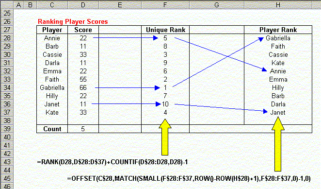
Here, we have 10 players, with 5 unique scores. In this example, the player names are sorted in alphabetical order. This is for illustration only. The players may appear in any order. To determine the ranking of the players, we first create their Unique Ranks, as described in the previous section. The formula we use for this is
=RANK(D28,D$28:D$37)+COUNTIF(D$28:D28,D28)-1
The next step is to pull the names out of the Player List (C28:C37) in the order determined by the ranks. To do this, we use the following array formula:
=OFFSET(C$28,MATCH(SMALL(F$28:F$37,ROW()-ROW(H$28)+1),F$28:F$37,0)-1,0)
Since this is an array formula, you must press Ctrl+Shift+Enter rather than just Enter when you first enter the formula, and whenever you edit it later. This formula uses several functions to extract the proper name from the list. To see how it works, lets look at the formula in H32, which returns "Annie". This formula is
=OFFSET(C$28,MATCH(SMALL(F$28:F$37,ROW()-ROW(H$28)+1),F$28:F$37,0)-1,0)
The code ROW()-ROW(H$28)+1 returns the position of the formula in the Player Rank range (H28:H37). It simply subtract the current row of H28 from the current row, and adds on. Since this formula appears in H32, this returns 5, as it is the 5th entry in the range. This value is passed to the SMALL function. SMALL returns the Nth smallest entry in the array it is passed. Since the 5th smallest entry in the list is 5, SMALL returns 5. This value is passed to the MATCH function, which tells us where in the Unique Rank list 5 appears. Since 5 appears first in the Unique Rank list, MATCH returns 1. Subtracting 1 from this and passing it to OFFSET, we get the first value from the Player List.
If you trace backwards following the arrows on the sample worksheet, it will become clear how the formula actually works.
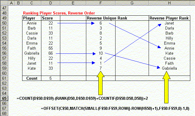
Ascending Player Ranking
If you need to rank players in ascending order (the "golfing" style), you can use the same procedures as the Descending Player Ranking section, but use the Reverse Unique Rank formula instead of the Unique Rank formula. The formulas for Ascending Player Ranking are summarized in the following sample worksheet:
Double Ranking
Double Ranking can be thought of a "tie-breaking" ranking. It is useful when you need to establish Unique Ranks for duplicate scores based on some other score. The Unique Rank formulas in earlier sections used the order in which the score appear to assign ranks. This may work in many situations, but not in others. For example, if you are ranking employees on sales amounts, you may want to break the ties based on seniority. That is, if two employees have the same sales amounts, the higher rank goes to the employee with the greater seniority.
To accomplish this, you'll need two tables of data, each listing the player and the score for that category. Then, you'll need to create a third table that assigns a "composite rank" based on the entries in the first two data tables. The following worksheet sample summarizes the data and formulas:
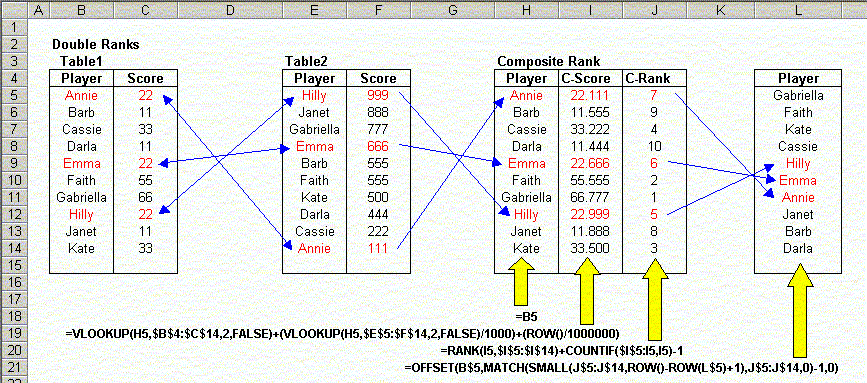
Here, we create the composite ranks, in column I, by
adding to the score in table 1 the score in table 2 divided by 1000, and then
the row number divided by 1,000,000. This ensures that the composite score
is unique for each player, even if the score in table 1 are the same.
(Adding the row number divided by 1,000,000 ensures that the composite scores
are unique even when there is a tie in Table 2. In this case, the formula we use
is
=VLOOKUP(H5,$B$4:$C$14,2,FALSE)+(VLOOKUP(H5,$E$5:$F$14,2,FALSE)/1000)+(ROW()/1000000)
Notice that since we use a VLOOKUP function to get the formulas from both tables 1 and 2, the players can appear in different orders in these tables. In this example, they are sorted by Name in Table 1 and sorted by Score in Table 2, but this is for illustration only. The names may appear in any order.
For example, look at players Annie, Emma, and Hilly, shown in red. Their Table 1 scores are all 22. To break the tie, we use their scores from Table 2. This is the composite score, shown in the C-Score column (column I). The C-Rank column (column J), uses our now-familiar Unique Rank formula to get the unique ranks of the Composite Scores.
Finally, the Players in column L are returned in the order of the composite ranks, using the same method described in the Descending Player Ranking section above.
If you follow the logic backwards, following the arrows, from column L to the the two score tables, the formulas will become clear.
Click here to download a workbook illustrating these formulas.