 List Functions
This page describes various formulas and VBA procedures for
working with lists of data.

There are a variety of methods and formulas that can be used with lists of data.
The examples that use two lists assume you have two named ranges,
List1 and List2, each
of which is one column wide and any number of rows tall. List1 and List2 must
contain the same number of rows, although the need not be the same rows. For
example, List1 = A1:A10 and List2 = K101:K110 is legal because the number of
rows is the same even though they are different rows.
You can download a example with these formula here.

For a VBA Function that returns a list of distinct values from a range or array, see the Distinct Values
Function page.
You can use a simple formula to extract the distinct elements in a list. Suppose
your list begins in cell C11. In some cell, enter
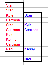
=IF(COUNTIF($C$11:C11,C11)=1,C11,"")
and then fill this formula down for as many rows as the number of rows in your data
list. This formula will list the distinct items in
the list beginning in cell
C11. In the image to the left, the original data is shown in red and the results
of the formula are shown in blue.
In the data shown in the image, the results are in a column adjacent to the original data.
This is for illustration only. The result data may be anywhere on the worksheet, or, for that matter,
on another worksheet or even in a separate workbook. The only restriction is that you must fill the formula down for at least as many
rows as there are in the data list.
See No Blanks for a formula to remove the blank cells in the result list to have all the
distinct entries appear at the top of the result list.
This formula assumes that the list that will contain the elements common to both
lists is a range named Common and that this range
has the same number of rows as List1 and
List2. This is an array formula that must be
array entered into a range of cells (see the Array
Formulas page for more information about array formulas). Select the range
Common and type (or paste) the following formula into the first cell, then press
CTRL SHIFT ENTER rather than just
ENTER. This is necessary since the formula
returns an array of values.
=IF(NOT(ISERROR(MATCH(List1,List2,0))),List1,"")
 The
result of this formula is an array of the values that exist in both
List1 and List2. The
positions of elements in the resulting list will be the same as the positions in
List1. For example, if List1
has 'abc' in its 3rd row and List2 has 'abc' in the 8th row, 'abc' will appear
in the 3rd row, not the 8th row, of the result list. If an element in
List1 does not exist in List2,
the element in Common of the unmatched item in
List1 will be empty.
The
result of this formula is an array of the values that exist in both
List1 and List2. The
positions of elements in the resulting list will be the same as the positions in
List1. For example, if List1
has 'abc' in its 3rd row and List2 has 'abc' in the 8th row, 'abc' will appear
in the 3rd row, not the 8th row, of the result list. If an element in
List1 does not exist in List2,
the element in Common of the unmatched item in
List1 will be empty.
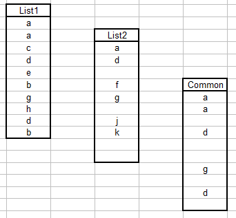
The image to the left illustrates several aspects discussed previously. First,
we have three named ranges, List1,
List2, and Common.
Second, all three ranges as the same size (10 rows in this case) but are all
different sets of rows. Finally, the position of the elements in the
Common range match the positions of elements in
List1, not List2.
You can also use a formula to extract elements that exist in one list but not
in
another. Again, it is assumed that you have two named ranges,
List1 and List2 of the
same size. Create a new named range called In1Not2
the same size as List1. Enter the followng formula in
the first cell of the new range ("In 1 Not 2") and press CTRL SHIFT
ENTER rather than ENTER. This is an array formula so it must be entered with
CTRL SHIFT ENTER rather than ENTER in order to work..
=IF(ISERROR(MATCH(List1,List2,0)),List1,"")
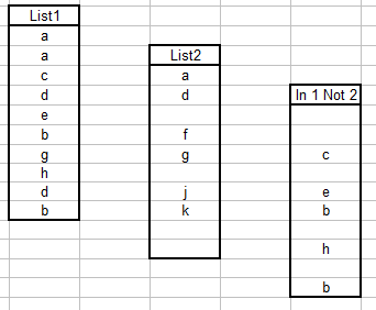 This
formula will return the elements in List1 that do not appear in
List2.
This
formula will return the elements in List1 that do not appear in
List2.
The order of the elements in the result list correspond to the position
of that element in List1.
You can use Excel's Conditional Formatting tool to highlight cells in a second list that appear or do not appear in a master list. Excel
does not allow you to reference other sheets in a Conditional Formatting formula, so you must use defined named. Name your master list
Master and name your second list, whose elements are to be conditionally formatted,
Second. Open the Conditional Formatting dialog from the Format menu. In that dialog, change
Cell Value Is to Formula Is. To highlight elements in the Second list that appear in the
Master list, use the formula
=COUNTIF(Master,OFFSET(Second,ROW()-ROW(Second),0))>0
To highlight cells that appear in Second but not in Master,
use Conditional Formatting as above but use the following formula:
=COUNTIF(Master,OFFSET(Second,ROW()-ROW(Second),0))=0
You can download a example with these formula here.
This page last updated:
14-July-2007