Weighted Average In Excel

In a normal average, each value to be included in the average with equal significance. For example, the uweighed average of 65, 60, 80, and 95 is (65+60+80+95)/4 or 75. A weighted average is an average in which one element may contribute more heavily to the final result than another element.

As an example, consider a university course in which the final grade is derived from the scores on two midterm exams, a score for homework, and the score on a final exam. However, the professor does not want to give equal weights to the values that go into the calculation of the final grades. The professor decides that homework should be give 2 times the significance of one midterm exam, and that the final exam is worth 3 times a single midterm. For this, you need to use a weighted average. If we assign a weight or significance of 1 to each midterm exam, the weight of the homework grade is 2 and the weight of the final exam is 3. Calculating the weighted average consists of multiplying each score by that score's weight, summing those products, and dividing not by the number of elements (as in an unweighted average) but by the sum of the weights. Continuing with the example we started with, suppose first midterm score in 65, the second midterm is 60, homework is 80, and the final exam is 95. This comes to a weighted average of(65*1 + 60*1 + 80*2 + 95*3)/(1+1+2+3) = 81.43. The unweighted average is 75. The weighted average is greater because the final exam (score 95) has three times the importance or weight of a midterm exam, and thus contributes more to the final grade.

Using the example above, suppose we have the scores in cells B6:E6 and the weights in cells B7:E7, as shown below:

weighted average

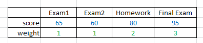
We can use the SUMPRODUCT function to multiply each score by its weight and then sum those products. Then, use SUM to add up the weights and finally divide the result of SUMPRODUCT by the sum of the weights:

=SUMPRODUCT(B6:E6,B7:E7)/SUM(B7:E7)

This gives us a result of 81.43.

This can be simplified if the sum of the weights in 1. For example, if we use as weights percentages, the weights in the example above become 14%, 14%, 29%, and 43%. (These values are calculated by dividing each weight by the sum of the weights.) Since these percentages sum to 100% or 1.0, we can omit the SUM function and simplify the formula to

=SUMPRODUCT(B6:E6,B7:E7)

This works because the sum of the weights is 1, so we are just eliminating the unnecessary division by 1.