 Flexible Lookups
This page describes formulas that provide greater functionality
than Excel's VLOOKUP and HLOOKUP functions.

Excel's built-in VLOOKUP and HLOOKUP
functions are great for simple table lookups. However, there are three basic shortcomings of these
functions. First, you can search for a match value only in the first column (or row) of the table range. Second,
you can return a value only from a column to the right of (or below) the lookup match column
(row). You can't return
a value to the left of a lookup value. Finally, VLOOKUP and HLOOKUP
can return only a single cell. This page describes formulas you can use to write much more
flexible lookup formulas.
Using a combination of OFFSET and MATCH functions
you can write a formula that uses any column of a data table for the lookup match, return a value from any
column of the data table, and return values from one or more adjacent columns in the data table. By way
of example, consider the following data table:
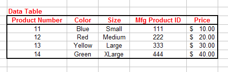
In this table, we define the name Table1 as the actual data region of the table,
not including the column headers. The formula for a flexible lookup function to replace
VLOOKUP, is as follows:
=IF(ISNA(OFFSET(Table1, MATCH(LookupValueV,OFFSET(Table1,0,
LookupColumnOffset,ROWS(Table1),1),0)-1,DataColumnOffset,ROWS(Table1),DataSizeV)),
"not found",OFFSET(Table1, MATCH(LookupValueV,OFFSET(Table1,0,LookupColumnOffset,
ROWS(Table1),1),0)-1,DataColumnOffset,ROWS(Table1),DataSizeV))
In this example formula, Table1 is the data table, excluding column headers.
LookupValueV is the value to search for in Table1.
LookupColumnOffset is the offset from the left column of
DataTable1 in which to search for LookupValueV. The
offset is 0-based, so a LookupColumnOffset of 0 searches the first column of
Table1. A value of 1 specifies that the second column
is to be searched, and so on. DataColumnOffset is the offset
from the left column of Table1 from which the return data values are to be taken. Like
LookupColumnOffset, the offset is 0-based, so a value of 0 returns values from the
first column of Table1, a value of 1 returns values from the second column, and so
on. DataSizeV is the number of columns of data, beginning in
LookupColumnOffset, to return.
Because the formula above can return more than one value, you must array enter it into several columns in a row. The number of
columns should be equal to the value of the DataSizeV. Select the cells in which the results
are to be returned, type or paste the formula above, and then press CTRL SHIFT ENTER rather than
just ENTER. If you do this properly, the formula will be entered in all of the selected cells.
Excel will display the formula in the Formual Bar enclosed in curly braces { }.
The formula will not work correctly if it is not entered with CTRL SHIFT ENTER
.
Array formulas are one of the most powerful tools in Excel. See the Introduction To Array Formulas
page for much more detail about array formulas.
In Excel 2007, a new function named IFERROR was added to Excel. This has the syntax:
=IFERROR(formula,result_if_error)
IFERROR evaluates formula and if there is no error, the result of formula is returned. If
formula results in an error, result_if_errror is returned instead of the actual error value (#N/A, for example). Before
the IFERROR was introduced, an error testing formula would be written like:
=IF(ISERROR(formula),result_if_error,formula)
You can easily see that formula is normally evaluated twice: once for the ISERROR function to see if it returns an
error and again to get the result if there is no error. This leads to a longer calculation cycle time. We can shorten the formula above to use
IFERROR
=IFERROR(OFFSET(Table1, MATCH(LookupValueV,OFFSET(Table1,0,LookupColumnOffset,
ROWS(Table1),1),0)-1,DataColumnOffset,ROWS(Table1),DataSizeV),"not found")
The formula above as written will return the results in a single row spanning several columns. If you need to return the results
into cells in a single column spanning several rows (the number of rows should be equal to the value of
DataSizeV), you need to transpose the result array. The following formula will do
this:
=IF(ISNA(TRANSPOSE(OFFSET(Table1, MATCH(LookupValueV,OFFSET(Table1,0,LookupColumnOffset,
ROWS(Table1),1),0)-1,DataColumnOffset,ROWS(Table1),DataSizeV))),"not found",
TRANSPOSE(OFFSET(Table1, MATCH(LookupValueV,OFFSET(Table1,0,LookupColumnOffset,
ROWS(Table1),1),0)-1,DataColumnOffset,ROWS(Table1),DataSizeV)))
This is the same function as the previous example, but uses the TRANSPOSE function to
transpose the result array. The parameters in this formula are exactly the same as those described in the earlier
formula. We can shorten this formula in Excel 2007 and later with the IFERROR function.
=IFERROR(OFFSET(Table2,DataRowOffset,MATCH(LookupValueH,
OFFSET(Table2,LookupRowOffset,0,1,COLUMNS(Table2)),0)-1,DataSizeH,1),"not found")
Again, replace not found, with the result to return if no match is found.
If LookupValueV is not found in the column specified by the
LookupColumnOffset, the function returns an array of strings whose values
are not found. If the array into which the function is entered is larger
than the number of values returned (the value of DataSizeV), the array is
filled out with #N/A error values. If the formula is entered into a range
of cells with fewer cells than the value of DataSizeV, the result array
is truncated to fill the cells into which the formula was entered.
Using the data table shown above, if LookupValueV is Yellow,
LookupColumnOffset is 1, DataColumnOffset is 0, and
DataSizeV is 4, the formula will return an array of values
13 Yellow Large 333 into four cells. These are the values, beginning in column offset
1 (the Color column), on the row on which Yellow was found, returning
DataSizeV = 4 values.
The formulas presented above are similar to the VLOOKUP
function in that they search down a column looking for a match, and then return a value from some column in row in which
the match was found. With a bit of revision, the formula can be adapted to perform like the
HLOOKUP function, which searches across a row and then returns a value
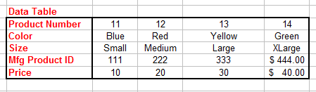
from some row in the column in which the match was found. Consider the following data table:
=IF(ISNA( OFFSET(Table2,DataRowOffset,MATCH(LookupValueH,OFFSET
(Table2,LookupRowOffset,0,1,COLUMNS(Table2)),0)-1,DataSizeH,1)),"not found",
OFFSET(Table2,DataRowOffset,MATCH(LookupValueH,
OFFSET(Table2,LookupRowOffset,0,1,COLUMNS(Table2)),0)-1,DataSizeH,1))
The parameters to this formula are essentially the same as those used in the example in the previous section.
Table2 is the data table, not including the row headers. LookupRowOffset
is the 0-based row offset from the top of Table2 that will be searched for
LookupValueH. DataRowOffset is the 0-based offset
from the top of Table2 of the starting row from which the values are to be retrieved.
DataSizeH is the number cells, starting in DataRowOffset, to
return. Using the example table above, if LookupValueH is Blue,
LookupRowOffset is 1, DataRowOffset is 0, and
DataSizeH is 3, the formula will return the following values to the cells in which it
is entered: 11 Blue Small.
This formua as written will return its results into cells in a single column, spanning several (DataSizeH)
rows. If you want to display the results in a single row spanning several columns, you must transpose the data
using the formula:
=TRANSPOSE(IF(ISNA( OFFSET(Table2,DataRowOffset,MATCH(LookupValueH,
OFFSET(Table2,LookupRowOffset,0,1,COLUMNS(Table2)),0)-1,DataSizeH,1)),"not found",
OFFSET(Table2,DataRowOffset,MATCH(LookupValueH,OFFSET(Table2,LookupRowOffset,0,1,
COLUMNS(Table2)),0)-1,DataSizeH,1)))
Remember, all of these formulas are array formulas, so you must first select
the cells into which the results will be returned, type the formula, and press CTRL SHIFT ENTER.
If you do not do this, the results will be incorrect.
 |
This page last updated: 3-April-2009. |