Excel is ideal for working with lists of data. This page describes a number of worksheet formulas for extracting basic information about a list -- sums, minimums, maximums, and so on. It also show you how to restrict these functions to only certain values in the list, such as values greater than zero, or values between two other values.
Also, there are a few formulas for transposing a list (changing a row into a column) and reversing the order of a list, or both. Finally there are a few miscellaneous formulas that didn't see to fit on other pages.
All of the formulas on this page are array formulas, so you must press Ctrl+Shift+Enter rather than just Enter when you enter the formula, and whenever you edit it later.
In this section, we will refer to a list of data named List. For more information about naming a range, click here.
You are already familiar with the basic SUM, MIN, MAX, and AVERAGE formulas, so they won't be explained here. Refer to the on-line help manual for basic information about these functions. Instead, for each function, use the function to use only the following values from List:
- Values Not Equal To Zero
- Values Greater Than Zero
- Values Between An Upper And Lower Limit
For example, you can find the average of those values in the List that are greater than zero, or between 10 and 20.
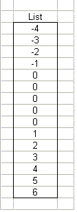
In all of these formulas, we will be using a range called List, which refers to the data show in the figure to the left.
Of course, your actual data will be different, and your List can be of any length. The values in this example will clearly show the different results when we're calculating the results using only non-zero values, or values between an upper and a lower limit.

Non-Zero Values
You can restrict the values used by the functions to only those values (positive and negative) that are not equal to zero. Remember, all these formulas are array formulas.
=SUM(IF(List<>0,List,FALSE))
returns the sum of non-zero values, or 11. Of course, summing non-zero
values is never really necessary (since the 0 values don't contribute to the sum
in any case), but the formula is illustrative nonetheless.
=AVERAGE(IF(List<>0,List,FALSE))
returns the average of non-zero values, or 1.1. If we used the AVERAGE
function on the entire list, the result would be 0.73, because the 5 zero values
would be included. In this function, they are not included.
=MIN(IF(List<>0,List,FALSE))
returns the minimum of non-zero values, or -4.
=MAX(IF(List<>0,List,FALSE))
returns the maximum of non-zero values, or 6.
Positive Values
You can restrict the values used by the functions to only positive values -- those that are greater than zero. Remember, all these formulas are array formulas.
=SUM(IF(List>0,List,FALSE))
returns the sum of positive values, or 21. The negative numbers are not
included in the sum.
=AVERAGE(IF(List>0,List,FALSE))
returns the average of positive values, or 3.5.
=MIN(IF(List>0,List,FALSE))
returns the minimum of positive values, or 1.
=MAX(IF(List>0,List,FALSE))
returns the maximum of positive values, or 6.
Values In An Interval
You can restrict the values used by the functions to only values between two other values. In these formulas, we will use two more named cells -- LLim which is the lower limit, and ULim, which is the upper limit. When we say "between" two numbers, we mean inclusively between. In other words, the numbers 2, 3, and 4 are all between 2 and 4. If you want to have the formulas work with exclusively between intervals (only the number 3 is between 2 and 4), change the <= and >= operators to < and >, respectively. Remember, all these formulas are array formulas. In the examples, assume that LLim contains 2 and ULim contains 5.
=SUM(IF((List>=LLim)*(List<=ULim),List,FALSE))
returns the sum of values between 2 and 5, or 14.
=AVERAGE(IF((List>=LLim)*(List<=ULim),List,FALSE))
returns the average of values between 2 and 5, or 3.5.
=MIN(IF((List>=LLim)*(List<=ULim),List,FALSE))
returns the minimum of values between 2 and 5, or 2.
=MAX(IF((List>=LLim)*(List<=ULim),List,FALSE))
returns the maximum of values between 2 and 5, or 5.
You can use array formulas to reverse the order of a list.
Reversing the Order Of A Column
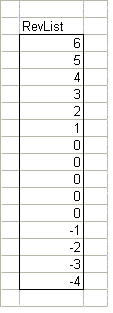
Still using the List from the previous section, we can reverse its order, which will give us the list shown below. This formula uses a named range called RevList, which refers to the range of the new, reversed list.
Enter this array formula in the first cell of the RevList range, then select the entire RevList range, and use Fill Down from the Edit menu to copy this formula down into all the cells in the RevList range. Remember this is an array formula.
=OFFSET(List,MAX(ROW(RevList))-ROW(),0)
This formula will work only for reversing the order of a column. To reverse the order of a row, see the next section.


